sEst example
loading the library and data (GSE51032)
library(sest)
Raw data files (.idat) for GSE51032 dataset were downloaded from GEO site (https://www.ncbi.nlm.nih.gov/geo/query/acc.cgi?acc=GSE51032). And, the raw beta-value and detection p-values were extracted using ‘minfi’ package (http://bioconductor.org/packages/release/bioc/html/minfi.html)
Assume that the matrix ‘beta.bg.XY’ has background-corrected beta-values (without any further normalization) for X-chromosome and Y-chromosome probes, and the matrix ‘p.XY’ has detection p-values for X-chromosome and Y-chromosome probes.
Sample QC, using the per-sample call-rate of chrX probes.
Assume that ‘QC’ is a data.frame with all the samples names in the GSE51032 dataset as rownames, and ‘callrate.X’ and ‘callrate.Y’ as colnames, which contains the proportion of probes with detection p-value <0.01 for chrX and chrY, respectively.
Let’s select for high-quality samples using the callrate.X of 0.95 as the cut-off.
samples.GSE51032.good <- rownames(QC[, "callrate.X"]>0.95)
Running sex-estimation
Calling ‘estimateSex’ function to estimate the sex-status of input data.
sex.GSE51032.good <- estimateSex(beta.value=beta.bg.XY[, samples.GSE51032.good], detecP=p.XY[, samples.GSE51032.good], return_with_reference=TRUE)
Contents of the ‘estimateSex’ result:
‘estimateSex’ returns a list object containing two data.frames: one is for reference data (‘reference’) and the other is for the test samples (‘test’)
names(sex.GSE51032.good)
[1] "test"      "reference"
head(sex.GSE51032.good$reference)
Sample| X.PC1 |Y.PC1 | predicted.X | predicted.Y | predicted
-
male.0001 -0.2537145 -0.6624954 M M M male.0002 -0.2798323 -0.6596785 M M M male.0003 -0.2161992 -0.6539044 M M M male.0004 -0.2597709 -0.6551377 M M M male.0005 -0.2542591 -0.6545710 M M M male.0006 -0.2634860 -0.6528368 M M M … … … … … …
head(sex.GSE51032.good$test)
Sample| X.PC1 |Y.PC1 | predicted.X | predicted.Y | predicted
-
6969568099_R02C02 0.1490050 0.3504673 F F F 6969568052_R02C01 0.1546120 0.4023443 F F F 6969568141_R03C01 0.1634140 0.2984963 F F F 6969568052_R01C02 0.1671693 0.3757989 F F F 7766130010_R05C01 0.1484081 0.5155788 F F F 6969568141_R06C02 0.1599462 0.4135742 F F F … … … … … …
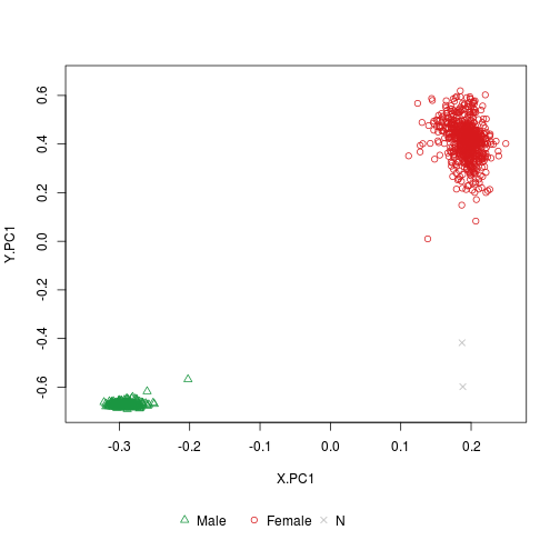
Plots of sex-estimation result
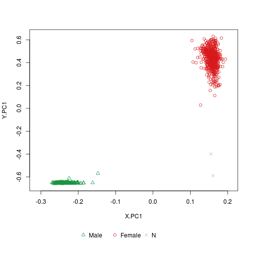
‘plotSexEstimation’: Shows the clustering of test samples with or without reference samples.
# without reference samples
plotSexEstimation(sex.GSE51032.good)
# with reference samples
plotSexEstimation(sex.GSE51032.good, include_reference = TRUE)
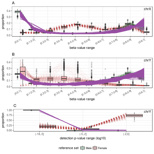
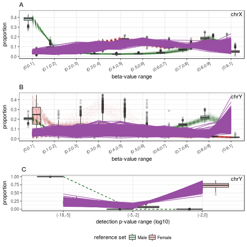
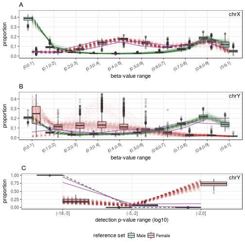
‘plotSexDistribution’: Shows the distribution profile of Male-predicted samples by :
# Male-predicted samples
samples.GSE51032.good.M <- rownames(sex.GSE51032.good$test)[sex.GSE51032.good$test$predicted == "M"]
plotSexDistribution(beta.value=beta.bg.XY, detecP=p.XY, samples=samples.GSE51032.good.M)
# Female-predicted samples
samples.GSE51032.good.F <- rownames(sex.GSE51032.good$test)[sex.GSE51032.good$test$predicted == "F"]
plotSexDistribution(beta.value=beta.bg.XY, detecP=p.XY, samples=samples.GSE51032.good.F)
# N-predicted samples
samples.GSE51032.good.N <- rownames(sex.GSE51032.good$test)[sex.GSE51032.good$test$predicted == "N"]
plotSexDistribution(beta.value=beta.bg.XY, detecP=p.XY, samples=samples.GSE51032.good.N)
Running sex-estimation with different beta-value intervals
Users can change ‘beta.intervals.X’ and ‘beta.intervals.Y’ to build beta-value distribution profiles with different beta-value intervals. The default is ‘seq(0,1,0.1)’. In the example codes below, ‘seq(0, 1, 0.2)’ is used as the beta-value intervals for both chrX and chrY. However, the estimation result is same.
sex.GSE51032.good.5 <- estimateSex(beta.value=beta.bg.XY[, samples.GSE51032.good], detecP=p.XY[, samples.GSE51032.good], return_with_reference=TRUE, beta.intervals.X = seq(0,1,0.2), beta.intervals.Y = seq(0,1,0.2))

plotSexEstimation(sex.GSE51032.good.5)
Although the beta-value intervals in this example use a fixed value for the increment, the increment value can vary. E.g., something like ‘beta.intervals.X = c(0, 0.2, 0.3, 0.4, 0.5, 0.6, 0.8, 1.0)’ is possible. Users can change the intervals of detection p-value too by using ‘p.intervals.X’ and/or ‘p.intervals.Y.’ options.